Backpropagation

Backpropagation is the central algorithm underlying neural network training. This post describes how it works and is split into three sections, covering:

• Perceptrons
• Multi-layered perceptrons
• Backpropagation

Intro

Though neural networks are recently popular, the central ideas underlying them were first published in the 1960s and 1970s.¹ We’ll start by reviewing perceptrons, which were invented in 1958 and behave much like a single node neural network.² Once we’re done with the perceptron, we’ll then move on to define a multi-layer perceptron, a class of neural networks. We’ll close with the algorithm needed to train such a network.

In all of the below formulations, we’ll be performing supervised machine learning. Given a pair $(\vec{x}, y)$, our goal will be to predict $y$. We’ll do this by learning a set of transformations that we can apply to input vector $\vec{x}$, which ultimately will output a prediction of $y$.

Perceptron

Definition

A perceptron is a tool for learning a threshold function for the purposes of making a binary classification. A perceptron is defined by:

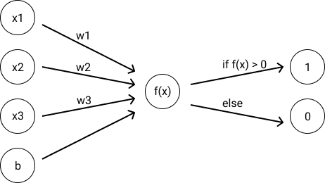
In the above, $\vec{w}$ is a vector of real-valued weights, $\vec{x}$ is an input vector, and $b$ is a real-valued scalar. The above produces a binary classification by computing the weighted sum of inputs plus some bias ($x_1w_1 + x_2w_2 ... + x_nw_n + b$) and then triggering if that value is greater than 0 and failing to trigger otherwise. One can visualize the computation of a perceptron below:

The if statement in the definition is what we’ll call an activation function, which will matter more later. An activation function takes the output of the previous step ($\vec{x} \cdot \vec{v} + b$) and transforms that intermediary into a final value.

Training

How do we train our model parameters ($\vec{w}, b$)?

Our goal is to choose weights to minimize prediction errors on our training data set. To do this, our approach will be to initialize our model’s weights to random values and to evaluate our model against every instance of our training data. After each evaluation, we’ll nudge our model’s weights in the right direction (just a little) when our predictions are wrong. We’ll stop this process either once our output error is below a threshold or until a predefined number of steps is complete.

How do we nudge our model weights in the right direction? To do this, we’ll manually choose a learning rate $\alpha$, which will be the size of our nudges. We’ll define our iteration number as $t$, and we’ll consider a training instance called $(\vec{x}, y )$ from our training set ($X$). For each $(\vec{x}, y ) \in X$, we’ll use the following rule to update our weights:

In other words, as we examine every training example in our data set, we’ll decrease $w_i$ slightly if our prediction was too low, and we’ll increase $w_i$ slightly if our prediction was too high. The magnitude of our increases or decreases will be proportional to how far off our prediction is, scaled down by a learning rate that we’ve manually chosen.

Drawbacks

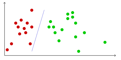
Perceptrons are limited in their power. In particular, the above training algorithm only converges to a set of stable weights if the training data is linearly separable. This is best visualized by imagining that we’re trying to classify points as either red or green; these points are linearly separable if a line exists that cleanly separates all red points to one side of the line or all green points to the other. To see why convergence is only guaranteed on linearly separable data sets, note that our model weights define a decision line, which will always imperfectly classify points if a line does not separate them.

Multi-layered perceptrons

Neural networks are multi-layered perceptrons. There are a few major differences between singleton perceptrons and multi-layered perceptrons:

• multiple perceptrons feed into one another to render a final prediction
• our activation function is a nonlinear function (e.g., the sigmoid), instead of an if statement as we saw above with the perceptron
• to account for the fact that our network is made of multiple perceptrons working together, our training step to update model weights is more complicated; we use backpropagation to learn weights.

Defining a neural network

Let’s define the important parameters of a neural network. We treat input vectors $\vec{x}$ as 1-indexed, reserving 0-indexing for biases. Definitions:

• $w^l_{ji}$ is a weight in a neural network’s graph. $j$ represents the index of a node in layer $l$ ,and $i$ represents the index of a node in layer $l - 1$.
• $W$ is an $N \times L$ matrix of weights, where $N$ is the number of nodes in each layer and $L$ is the number of layers.
• $g$ is an activation function, which could be any number of functions including a sigmoid, softmax, or other nonlinear $\mathbb{R} \rightarrow \mathbb{R}$ function
• $w^l_{j0}$ is used to represent the additive bias term for node $j$ in layer $l$ for $l < L$.

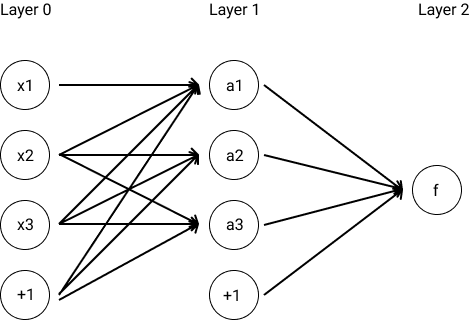
Below is an example neural network. It looks a lot like a perceptron. Note that the zero-indexed bias terms ($w^l_{j0}$) are represented by the nodes labeled +1. The middle layer (i.e., layer 1) is known as a hidden layer.

To compute the neural network’s output in the above example, we take $g(\sum_{i=0}^3 w^2_{1i}a_i)$, where each $a_i = g(\sum_{j=0}^3 w^1_{ij}x_j)$. These two summations represent the final layer’s computations and the middle layer’s computations, respectively.

Generalizing, a neural network performs a perceptron-like computation at each node, where the input vector is the result of the previous layer’s nodes. More formally, the output at node $j$ in layer $l$ takes the form:

Note that a neural network’s full prediction $f(x) = a_1^L$ in the above notation.

Activation functions

Neural networks make use of several different activation functions. Wikipedia notes that a logistic function is often used for binary classification; softmax is often used for multi-class classification in the final layer with logistic functions being used for inner layers; and other functions (including ReLU) are common.

An important point about activation functions is that neural networks are only really useful if activation functions are nonlinear. Compositions of linear functions are themselves linear, meaning that if we were to use linear activation functions, our entire neural network would collapse into a simple linear model: we’d be computing the following sum of $x$’s components. Nonlinear activation is essential to making neural networks interesting.

Backpropagation

Fundamentally, backpropagation is “little more than an extremely judicious application of the chain rule and gradient descent”³.

Minimizing error

We train neural networks much like we would train perceptrons: we iterate through each data point in our training set, evaluate our model’s prediction for that data point, and correct our model’s weights to reduce prediction error. Because of the layered, compositional nature of neural networks, our training step requires a bit more subtlety than our perceptron’s training step.

While training weights, we are trying to minimize an error function, which we’ll call $E(X, W)$, where $X$ is our training data set and $W$ is our model parameters (i.e., edge weights). As was the case with our activation function, our error function can take many forms. For learning a continuous function, we might use squared loss, as in $E(X, W) = \sum_{\vec{x} \in X} \frac{1}{2} (f(\vec{x}) - y)^2$. Other popular loss functions include negative log likelihood or cross entropy loss.⁴ Once we fix an error function, we update model weights according to:⁵

where $W^t$ represents the parameters of the neural network at iteration step $t$. In words, we update our model parameters by subtracting a scaled version of a matrix representing the gradient of our error function. Namely, it is a matrix where entry $(i, j)$ is the partial derivative of our error function with respect to $w_{i,j}$. This step is spiritually similar to our perceptron update rule in that our parameter nudges are proportional to the magnitude in error improvement that we expect from a nudge. This process is known as gradient descent.

Computing nudges efficiently

We’ll break our algorithm into two stages:

• Forward phase
• Backward phase

The purpose of the forward phase is to evaluate the model’s current prediction on an input; while doing so, we’ll compute a set of intermediary values that will be useful during the backward phase. During the backward phase, we’ll be able to compute the gradient of our error function, which will then enable us to update our weights accordingly.

We’ll run through the algorithm for a neural network predicting a continuous value, using the sigmoid as our activation function for all hidden layers (i.e., $g(x) = \frac{1}{1+e^{-x}}$) and the identity function for our final layer (i.e., $g(x) = x$). Note that this presentation was heavily inspired by the formulation presented on Brilliant, so check out their formulation if this one confuses you.

Forward phase

For each example in our training data, compute the network’s output $y' = f(\vec{x})$. Start from the first layer, feeding forward throughout the network to compute $f(\vec{x})$. Along the way, store the final output $f(\vec{x})$ and the following intermediary values for all nodes $i$ in layer $l$:

• $z_i^l = \sum_{j=0}^N w^l_{ij}a^{l-1}_j$, the sum of a node’s inputs
• $a_i^l = g(z_i^l)$, the activated sum of a node’s inputs

Backward phase

The goal of the backward phase is to compute the partial derivative of our error function with respect to each weight in our neural network; we want to do this for all networks weights, for all examples in our training data.

We’ll start by computing the partial derivative of our error function for our final output node in layer L. Next, we’ll use intermediary computations from computing layer L’s partial derivatives to compute layer L-1’s partial derivatives and so on back until the first layer. Below, all computations assume a squared loss function, a sigmoid activation function ($g(x) = \frac{1}{1+e^{-x}}$) for hidden layers, and an identity function for the final layer’s activation. We consider computations for a single training example $(x, y)$ with input $x$ and label $y$.

For our final layer, we compute:

For node $i$ in layer $l$ where $0 \leq l < L$, we compute:

Proof of formulas

The above formulas fall out of the chain rule, which tells us that: $\frac{\partial E}{\partial w^l_{ij}} = \frac{\partial E}{\partial z^{l}_{i}} \frac{\partial z_i^{l}}{\partial w^l_{ij}}$

We’ll work on deriving the first term in the above chain-ruled equation ($\frac{\partial E}{\partial z^{l}_{i}}$) first.

• First term, case 1: For the final layer in the neural network, we can differentiate our error function directly with respect to its summed inputs $z^L_1$. This means differentiating $\frac{1}{2}(g(z^L_1)-y)^2$ with respect to $z^L_1$, which gives us $g'(z^L_1)(g(z^L_1)- y)$. Because the derivative of the identity function is 1, and the identity function is our final layer’s activation function, this formula becomes $(g(z^L_1) - y)$ or simply $(y' - y)$.

• First term, case 2: For the hidden layer in the neural network, we again apply the chain rule and remember that our activation function is the sigmoid, where $g'(x) = g(x)(1-g(x))$. We define $\delta^l_i$ for later recursive use:

  $$\begin{align} \delta^l_i &= \frac{\partial E}{\partial z^l_i} \\ &= \sum_{k=0}^N \frac{\partial E}{\partial z_k^{l+1}} \frac{\partial z_k^{l+1}}{\partial z^l_{i}} \\ &= \sum_{k=0}^N \delta^{l+1}_k \frac{\partial z_k^{l+1}}{\partial z^l_{i}} \\ &= \sum_{k=0}^N \delta^{l+1}_k \frac{\partial(\sum_{m=0}^N w^{l+1}_{km}g(z_m^l))}{\partial z_{i}^l} \\ &= \sum_{k=0}^N \delta^{l+1}_k w^{l+1}_{ki}g'(z^l_i) \\ &= g'(z^l_i) \sum_{k=0}^N \delta^{l+1}_k w^{l+1}_{ki} \\ &= g(z^l_i)(1-g(z^l_i)) \sum_{k=0}^N \delta^{l+1}_k w^{l+1}_{ki} \\ &= a_i^l(1-a^l_i) \sum_{k=0}^N \delta^{l+1}_k w^{l+1}_{ki} \end{align}$$

• Second term: the second term in our chain-rule equation is the same for our hidden layers and our final layers. To compute $\frac{\partial z_i^{l}}{\partial w^l_{ij}}$, note that:

When differentiating the above with respect to $w^l_{ij}$, all terms in the summation go to zero except for $w^l_{ij}a_j^{l-1}$, which when differentiated equals $a_i^{l-1}$.

Updating weights

We just computed the partial derivative of our error function with respect to each weight in our neural network. We now take the simple average of these partial derivatives across all training examples, and update weight $w^l_{ij}$ by taking a step along the negative gradient. The size of our step will be scaled by our learning rate $\alpha$.

In short, we’ll execute:

Footnotes